n3He - Simulations

2006-11-30

Chopper simulation report

2007-10-01

Simulation of geometry factors, ignoring transverse dimensions of chamber (n3he_sim.pdf)

2007-10-04

FNPB Supermirror Polarizer report

2013-02-27

Simulation on ionization current in each wire (ion_current.pdf, ion_current.docx)

2014-03-24

Geometry Factors Part I PDF

2014-07-02

Statistics Report PDF

2014-07-22

Beam intensity fluctuations' effect on asymmetry uncertainty in n3He by David Bowman (n3Heintensityfluctuations.pdf)

2014-07-30

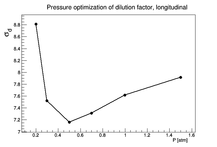
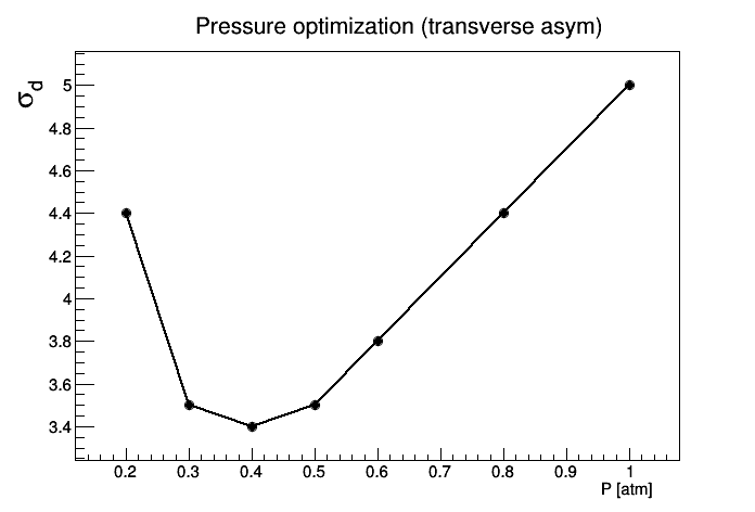
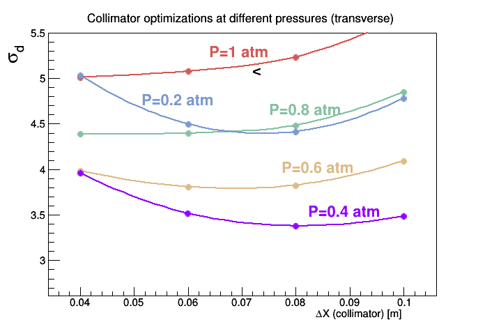
Preliminary results from improved simulation (v1.17, mcstas file) for longitudinal and transverse simulations. The optimal pressure from these results is 0.5 atm. In longitudinal mode it is a shallow minimum, but in transverse mode there is an improvement of 40% in reducing the pressure. At the minimum the transverse dilution factor is 2x smaller than longitudinal.

Longitudinal polarization:

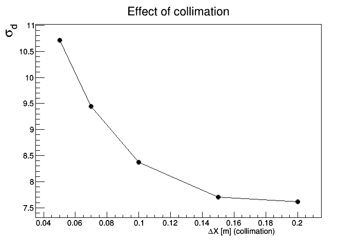
Transverse polarization:

2014-07-31 Geant4 Simulation (web)

2014-10-15 Centroid Analysis PDF

2014-11-11 Geometry Factors part II PDF

2015-01-05 GEANT4 Dilution Factor Simulation Results (Gericke)

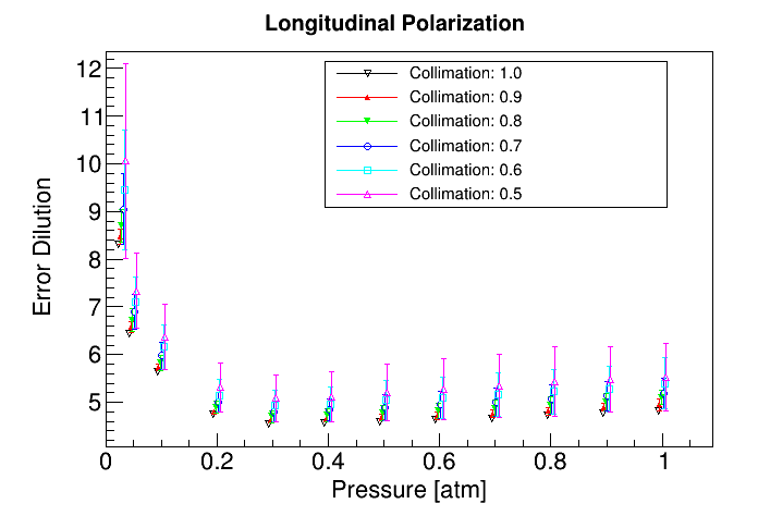
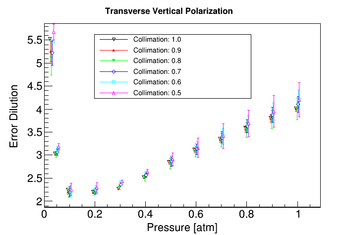
Shown below are the results of a simulation of the dilution factor and error using GEANT4 code. I performed 5 duplicates of 72 runs for 12 pressure settings and 6 different collimation
settings for both, the transverse and longitudinal polarization direction, as shown in the plots below. Each run had 5 million primary events (started neutrons), for a total of 1.8e9 simulated neutrons.
The analysis / calculation of the dilution factors and the errors is identical to that used by Chris Crawford. The error bars shown on the plots were obtained by starting each run of 5 million events with a
different random seed, which was itself randomly selected using the RanecuEngine (runs could be repeated with different engines to check systematic dependence on the seed generation). For each
pressure and collimation configuration the error in the simulated dilution and error was computed from the variance between the 5 runs (better errors can be obtained by running more repetitions of the 72
pressure and collimation configurations). Large error bars indicate there are large fluctuations between statistically independent runs with the same configuration.

The data points in the plots are slightly offset with respect to each other along the pressure axis to facilitate visualization. The simulated pressures are (in atm) 1, 0.9,
0.8, 0.7, 0.6, 0.5, 0.4, 0.3, 0.2, 0.1, 0.05, and 0.03. The simulated collimation was (in fraction of a 12 cm beam along the vertical) 1.0, 0.9, 0.8, 0.7, 0.6, and 0.5. The wire cell geometry in the simulation
was implemented as build.

Observations:

1) For longitudinal polarization, the dilution factor is much lower than that found by Chris Crawford and has a much less drastic dependence on the pressure above 0.2 atm. For high collimation the simuation errors are too large to tell if there is any meaning full dependence on the collimation, except at very low pressures. For a less collimated beam there appears to be a very slight dependence on collimation, but not a significant one. There is a shallow minimum at 0.3 atm, which seems to agree with the results obtained by Chris Crawford.

2) For vertical transverse polarization the dependence on pressure is much more pronounced and the minimum dilution (at 0.2 atm, rather than 0.4) is about factor of two lower than it is for longitudinal polarization which agrees with Chris Crawford's results. The error bars are significantly smaller, suggesting that this configuration may provide a more stable operating mode.

More runs with different random seeds could be performed to verify these results.

A more detailed write up of these simulations, including benchmarking data and geometrical configuarion will be provided later.

2015-03-12 Geometry Factors

Simulation results at 0.5 atm, with 8 cm collimation (transverse L/R asymmetry), and averaged over all TOF bins.
The first table "beta_i" is ion yield per cell, the second "gamma_i" is the geometry factors, and the third "weight_i" is the optimal weight of each wire asymmetry in the final extraction. See code, and mcstas ntuple. (note: I used an alternate mcstas ntuple to generate these results, but the other is a better representation of the polarizer). Note that almost all of the weight is in the outer two wires. (the shorted wire is 3rd from the end, which is good). The 2x4 block (outer 2 wires in the first 4 rows) carries 1/3 of the effective statistics on each side. Although the outside wire has a geometry factor of 80% vs 62% for the 2nd wire, the 2nd wire sees more capture events and therefore has a higher sensitivity to the physics asymmetry. Also attached is the mcstas.root file used to generate events up to the end of the guide (just before the polarimeter).

2015-04-02 Covariance Matrix

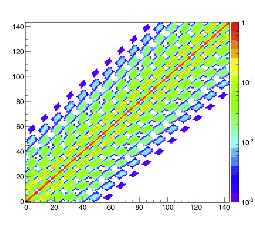
The full covariance matrix associated with the simulation above (2015-03-12). beta_i are the same numbers as above, but all on one line (use this data to correlated positions in this 1-d array, which (row,col) in the 2-d array above. beta_ij = < beta_i beta_j > = Cov(N_i, N_j) / N of Eq. 9 in (n3he_sim.pdf). N_i is the number of ions detected in the i'th cell due to captures from all N neutrons of one pulse.

2015-04-07 Analysis Meeting

We met and Chris explained his MC simulation, and write-up. See notes .

2015-06-03 Correlations

See Carlos's presentation on correlations. Here is a plot of the MC correlations of signals (not asymmetries). It does not include detector normalization, but there are no beam fluctuations in MC.

2015-06-24

Chris Coppola's updated simulation report.

2015-11-08

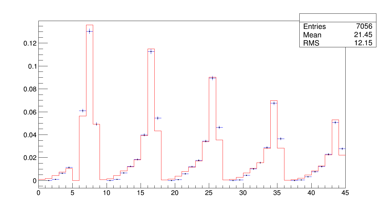
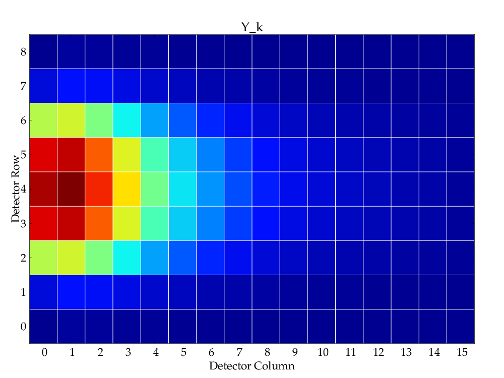
Here are some outputs from the MC simulation. Yields, geometry factors, weights, and correlations.
P = 0.476atm, c = 8.2cm, N = 2.15e9. sigma_d = 3.19
Time structure has been summed to simplify analysis and comparisons. I can provide time-resolved values on request.
Some corrections and refinements remain to be implemented.
- Chris Coppola

2015-12-16

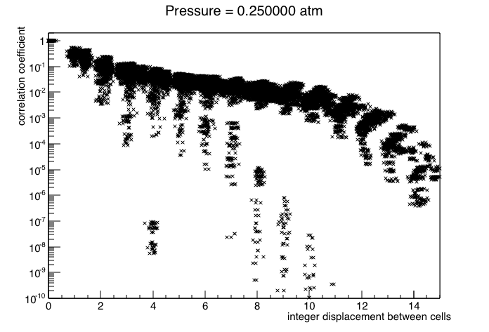
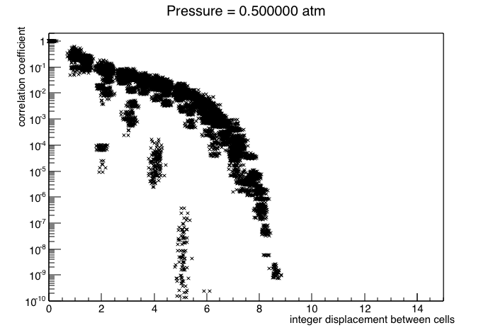
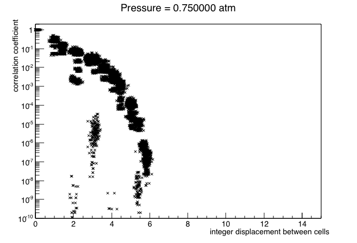
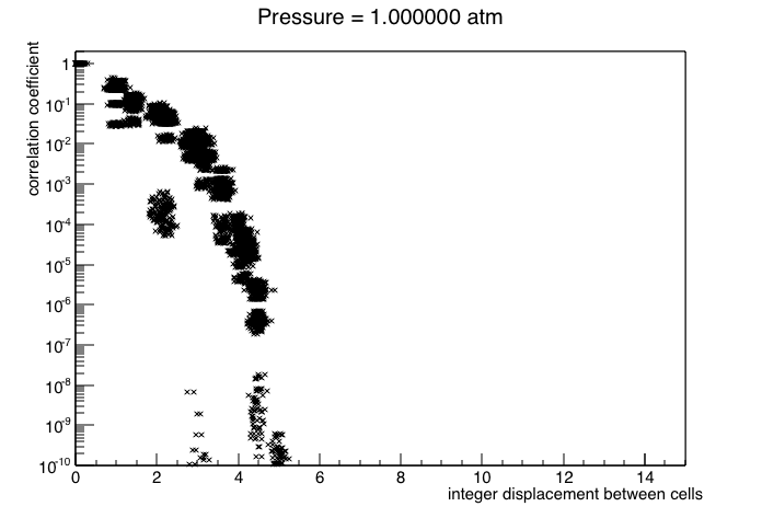
Here are the correlation matrices from my simulation at different. They are L/R geometry factors (transverse spin up/down), with x_col=8cm, only 1 TOF bin, using all 101901 events from poly_si6/b45/mcstas.root, with my updated simulation det3d_n3he.C~1.30. For each pressure, I include two files: one with the same information as above merged into one file, and the other with correlations alone, directly readable in Matlab, or the free web-app octave-online. Here are the octave commands used to extract the correlations from the covariance matrix: octave:> load c25.mat; d=diag(c25); r25=c25./sqrt(d*d'); save r25.mat r25

0.25 atm: simulation, correlation; 0.5 atm: simulation, correlation; 0.75 atm: simulation, correlation; 1 atm: simulation, correlation

0.25 atm

0.5 atm

0.75 atm

1.0 atm

For 1 atm, in my simulation, the maximum range was hardcoded to 7 cm = 3.68 cell widths. This maximum corresponds to a maximum displacement of (2,3) or (3,2) from one corner of a cell to the next, which would be at disp=sqrt(3^2+4^2)=5 on the plot (centre to centre). You can see the maximum in the plot is slightly higher because I dithered up to 0.1 in the x-direction to see individual points. The correlations below the main curve are low statistics in the simulation and cells on the side for which much fewer events came.

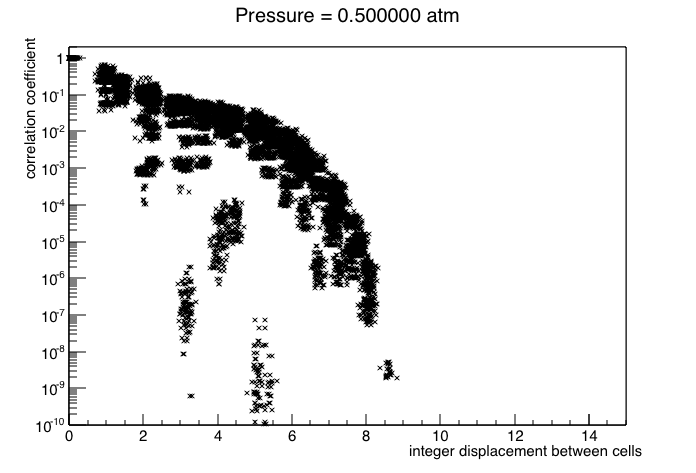
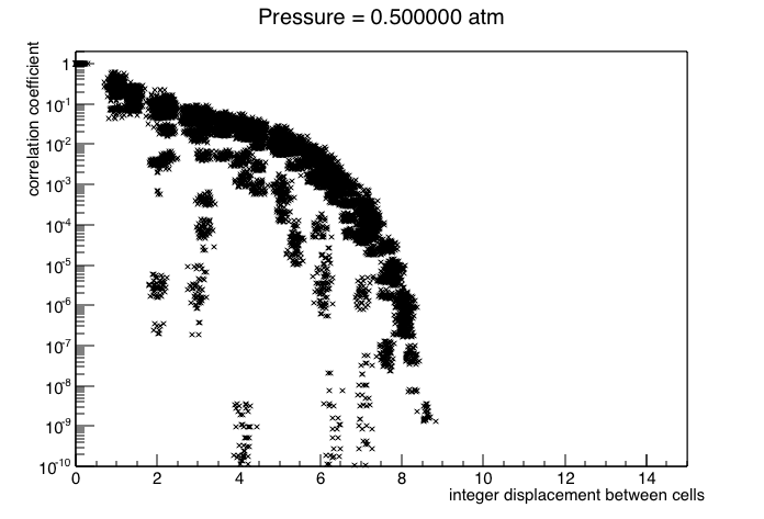
Here are the geometry factors and same plots for 0.5 atm, but collimation reduced from 8 cm to:

4 cm: simulation, correlation; 6 cm: simulation, correlation

4 cm collimation

6 cm collimation

2016-10-04

Comparison of MC and exp for collimation scans for Run 37990 (2nd from top of vertical scan). For this scan, the y-colimators were set at 21.7 and 19.7 cm; the beam center was at 15.1 cm. So I used the values xcol= (21.7-19.7)/100cm = 0.002 (full width) and x0col = ((21.7+19.7)/2 - 15.1) /100cm = 0.056
(center of swath). I ran this simulation with on the mcstas file . Here is the log of the simulation. Then I used this script to compare the result with Kabir's processed data files . Here is the log. Note that the chamber in my simulation is hard-coded in the L/R direction, so I actually set the x-collimator, not the y-collimator. Note that the error bars are meaningless!